SIGMOID Activation Function
When we are building a neural network almost always the
function we want to model is not linear in nature. To deal with this we need to
use an activation function which introduces non-linearity into the neural
network. A common activation function uses the SIGMOID function, define by the
equation below.

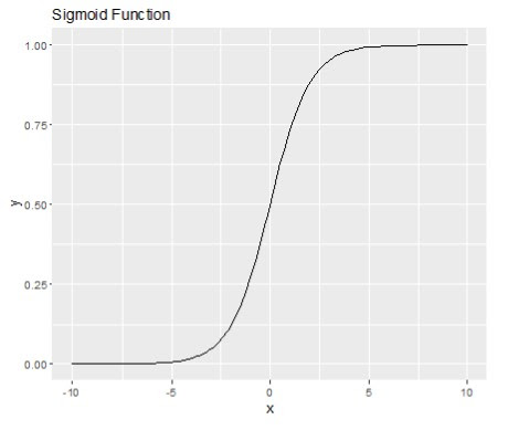
For a given value of x the SIGMOID function will produce an output
between 0 and 1. We can demonstrate this with the following R code.
library(ggplot2)
# Define sigmoid function
sigmoid <- function(x) {
1 / (1 + exp(-x))
}
# Generate data
x <- seq(-10, 10, length.out = 100)
y <- sigmoid(x)
# Create data frame
df <- data.frame(x = x, y = y)
# Plot sigmoid function
ggplot(df, aes(x, y)) + geom_line() + labs(title =
"Sigmoid Function", x = "x", y = "y")
Adding a weight to the SIGMOID
By adding a weight W to the sigmoid equation we can vary the
gradient of the slope between 0 and 1, as shown but the R code below.

library(ggplot2)
x <- seq(-10, 10, length.out = 1000)
# Define sigmoid function
sigmoid <- function(x) {
1 / (1 + exp(-x))
}
# Generate sigmoid curves for different constants
constants <- c(0.5, 1, 1.5, 2)
curves <- lapply(constants, function(c) sigmoid(c * x))
# Plot the curves
ggplot() +
geom_line(aes(x,
curves[[1]], color = "0.5")) +
geom_line(aes(x,
curves[[2]], color = "1")) +
geom_line(aes(x,
curves[[3]], color = "1.5")) +
geom_line(aes(x,
curves[[4]], color = "2")) +
ggtitle("Sigmoid Function with Varying Slopes") +
xlab("x")
+
ylab("y")
+
scale_color_manual(values = c("0.5" = "blue",
"1" = "red", "1.5" = "green",
"2" = "purple")) +
theme_bw()

Bias connection
We can add another input to the activation function called
bias input. Bias input is always one multiplied by a weight b. The purpose of
the bias input is to move the sigmoid function either to the left or to the
right as by the R code shown below.

sigmoid <- function(x, bias) {
1 / (1 + exp(-x +
bias))
}
# Set up plot
plot(NULL, xlim = c(-10, 10), ylim = c(0, 1), xlab =
"x", ylab = "y")
# Plot sigmoid curves with different biases
curve(sigmoid(x, bias = -3), add = TRUE, col =
"blue", lwd = 2)
curve(sigmoid(x, bias = 0), add = TRUE, col =
"red", lwd = 2)
curve(sigmoid(x, bias = 3), add = TRUE, col =
"green", lwd = 2)
# Add legend
legend("topleft", legend = c("-3",
"0", "3"), col = c("blue", "red",
"green"), lwd = 2)

Logistic Regression
The Sigmoid function can be used to calculate logistic
regression. This kind of regression is used to calculate the probability of a
binary outcome or decision based on the input.


